On the recognition of concert halls by room acoustics - Results of the first online listening experiment.

(NOTE: THERE IS NOW A SECOND VERSION OF THIS ONLINE LISTENING EXPERIMENT.)

Last September (2020) we published the article “Recognizing individual concert halls is difficult when listening to the acoustics with different musical passages”. The title already tells a lot of this experiment, where the subjects were required to recognize halls just by listening to the room acoustics, but so that the sounds (i.e. excitations) were either exactly the same or different. The sound materials included an excerpt of a Beethoven symphony, and short samples of a single violin (see the article for more details).

The following figures summarise the main results presented in the article:

FIG. 6. Overall results: The mean proportion of correct answers with confidence intervals derived from the binomial distribution with normal approxi- mation. Data are pooled over all individuals and each observation is treated as an independent binary (correct/incorrect) observation.

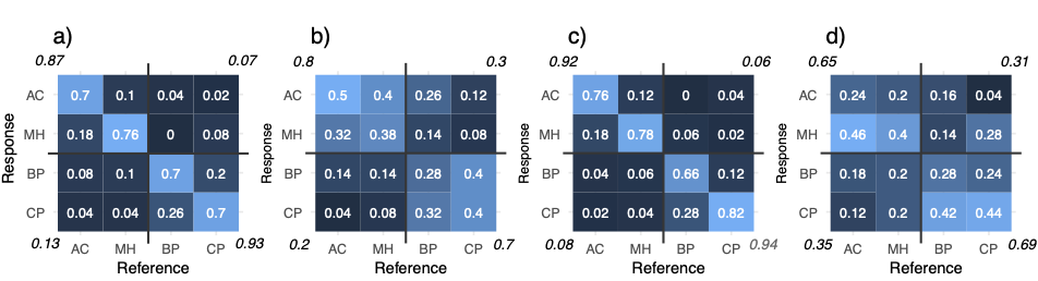FIG. 7. Confusion matrices (or “error” matrices) where each cell depicts the proportions (between 0 and 1) of responses given in the matching task. For example, in (a) whenever a reference auralization corresponded to AC, 70% of the responses were correct, while in 18% the response was incor- rectly MH. The values in the corners present the results of the reclassification of the correct responses with horizontal and vertical lines across the matrices indicating the grouping (i.e., AC–MH vs BP–CP, see text for details). (a) Beethoven “same” condition; (b) Beethoven “different” condition; (c) violin “same” condition; (d) violin “different” condition. Color range is scaled from 0 (dark blue) to 1 (white).

In any case, the story is that for this work I also experimented with RShiny to see if it can be used for making online listening experiments. Originally the idea was only to facilitate the review process, so that, the reviewers could go and have a listen for themselves. Here is link to this online test.

The online test was basically a copy of the live experiment (with some number of extra unknown variables), but unfortunately, i feel that it was excessively long to be directly transferred online. I suspect that there have been quite a lot of people who may have started the test but never completed. But I am happy to note that there are now as much as 40 people who have taken the time and completed. This amounts to a dataset, that can be summarized as follows:

# First remove variables from workspace
rm(list = ls()) 
# and read the data.table:
chm_df <- read.table("RSHINYresults.txt", sep = ",", header = T,stringsAsFactors = T)
summary(chm_df)

##      SUB_ID          ORD           CASE_ID      SOUNDTYPE      SOUNDNUM    
##  4GwhMP :  32   Min.   : 1.00   Min.   : 1.00   INSTR:640   Min.   : 0.00  
##  56IycUX:  32   1st Qu.: 8.75   1st Qu.: 8.75   MUSIC:640   1st Qu.: 0.00  
##  5QG    :  32   Median :16.50   Median :16.50               Median : 0.50  
##  5WsqUN :  32   Mean   :16.50   Mean   :16.50               Mean   : 4.25  
##  HAYtW  :  32   3rd Qu.:24.25   3rd Qu.:24.25               3rd Qu.: 8.25  
##  HKzhS7 :  32   Max.   :32.00   Max.   :32.00               Max.   :16.00  
##  (Other):1088                                                              
##  SAMEDIFF     MUS_REF       MUS_COM    REF       A        B        C      
##  diff:640   BEE1  :320   BEE1   :320   AC:320   AC:301   AC:322   AC:317  
##  same:640   BEE2  :320   BEE2   :320   BP:320   BP:325   BP:307   BP:318  
##             viulut:640   viulut :320   CP:320   CP:347   CP:299   CP:327  
##                          viulut2:320   MH:320   MH:307   MH:352   MH:318  
##                                                                           
##                                                                           
##                                                                           
##   D       ANS         CORRECT                        TIME        COMPLETED
##  AC:340   AC:304   Min.   :0.0000   2020-11-02 11:28:29:   1   Min.   :0  
##  BP:330   BP:339   1st Qu.:0.0000   2020-11-02 11:31:09:   1   1st Qu.:0  
##  CP:307   CP:350   Median :0.0000   2020-11-02 11:32:28:   1   Median :0  
##  MH:303   MH:287   Mean   :0.3852   2020-11-02 11:33:53:   1   Mean   :0  
##                    3rd Qu.:1.0000   2020-11-02 11:35:16:   1   3rd Qu.:0  
##                    Max.   :1.0000   2020-11-02 11:35:49:   1   Max.   :0  
##                                     (Other)            :1274              
##       REP             EXPERTICE             HEADPHONE  
##  Min.   :0.00   experienced:512   AKG 240DF      : 32  
##  1st Qu.:0.75   expert     :192   AKG K240 Studio: 32  
##  Median :1.00   none       : 96   AKG K501       : 32  
##  Mean   :0.75   novice     :416   AKG801         : 32  
##  3rd Qu.:1.00   NA's       : 64   AirPod Pro     : 32  
##  Max.   :1.00                     (Other)        :800  
##                                   NA's           :320

(You can download this dataset here .)

In total we have now 1280 data points, and I think this is fair amount of data to skim through. Note, that analyzing this type if data in R was already discussed in the previous post, so here, I will just cover the main results of the online listening experiment.

So, here are the results (in the similar figures as in the article):

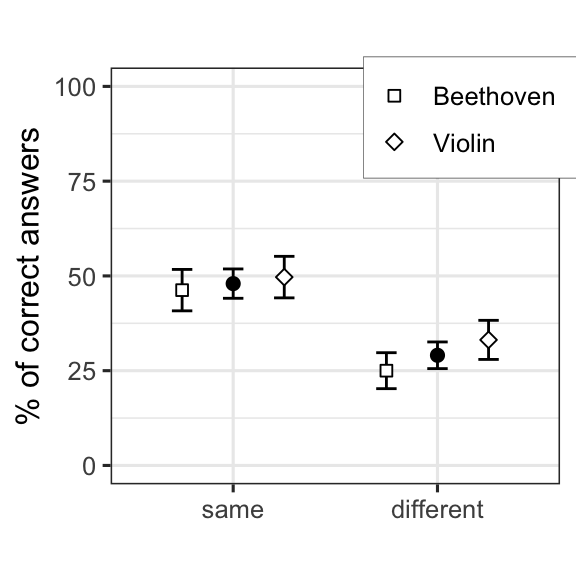
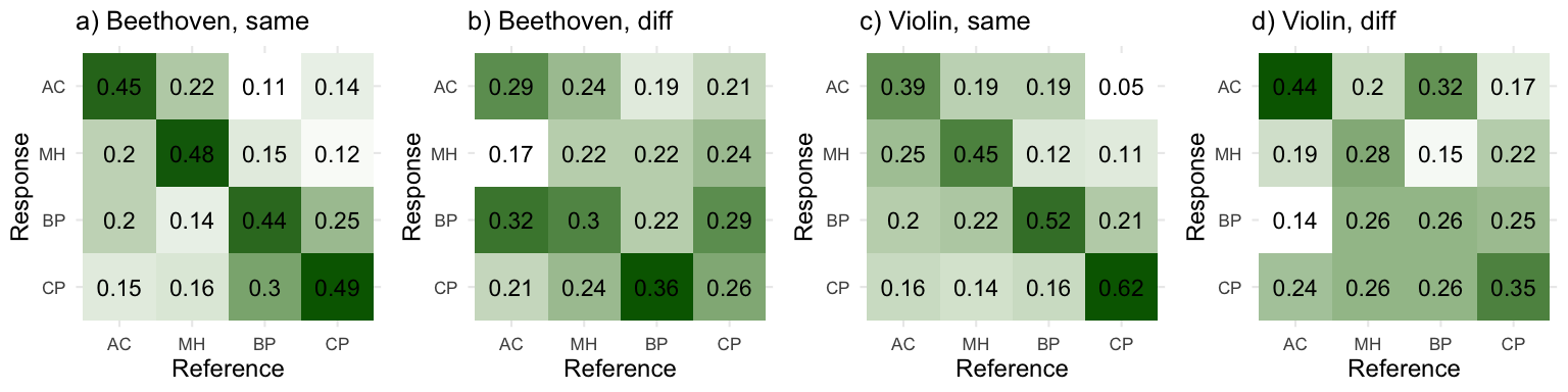
So, basically these results follow those presented in the article, but they are much worse. As mentioned, the test was relatively long to be performed online, so I suspect that these results are affected by the length of the experiment. Of course there is also the fact that the stimuli in the online test were binaural auralizations while the main experiment was carried out in the multichannel anechoic listening chamber at the Aalto Acoustics Lab. The multichannel chamber and the reproduction setup is critical when it comes to perceptually analysing small changes in the sound, and when listening to these samples myself, I can say that the binaural stimuli makes the task that more difficult.

Nevertheless, these results are in line with the article, and indicate that the recognition task was much more difficult when the sounds were different, than when they were the same. This can also be quantified with the binomial tests. (We make the assumption that all trials are independent, which is perhaps not strictly true.)

Exact binomial test for the “same”-condition:

## 
##  Exact binomial test
## 
## data:  same_corn and same_totn
## number of successes = 307, number of trials = 640, p-value < 2.2e-16
## alternative hypothesis: true probability of success is greater than 0.25
## 95 percent confidence interval:
##  0.4465431 1.0000000
## sample estimates:
## probability of success 
##              0.4796875

Exact binomial test for the “diff”-condition:

## 
##  Exact binomial test
## 
## data:  diff_corn and diff_totn
## number of successes = 186, number of trials = 640, p-value = 0.01081
## alternative hypothesis: true probability of success is greater than 0.25
## 95 percent confidence interval:
##  0.2610833 1.0000000
## sample estimates:
## probability of success 
##               0.290625

These results show clearly that people could recognize the halls above the level of chance (i.e., 1/4) in the “same” -condition. In the “diff”-condition, the result is still significant with p-value of 0.01, so it seems not to be totally random and people could perhaps tease out the correct hall, but not very consistently. Looking at the figures, there also seems to be a small difference between the Beethoven and violin in the “diff”-conditions.

The contrast between the “same” and “diff” conditions is perhaps self-evident, but we can still verify it by testing whether the two proportions are equal or not. We use the Chi-Squared test for two proportions:

## 
##  2-sample test for given proportions with continuity correction
## 
## data:  c(same_corn, diff_corn) out of c(same_totn, diff_totn), null probabilities c(1/4, 1/4)
## X-squared = 184.27, df = 2, p-value < 2.2e-16
## alternative hypothesis: two.sided
## null values:
## prop 1 prop 2 
##   0.25   0.25 
## sample estimates:
##    prop 1    prop 2 
## 0.4796875 0.2906250

As mentioned, this online experiment was excessively long, so I don’t continue with any further analyses here.

You can download this dataset here if you want to take a closer look.

Finally, I am still continuing this research with another experiment, that includes another set of sounds and is now considerably shorter. Please participate!.

Leave a comment: